Sampling from a Gaussian Process

Given a Gaussian Process (GP) specified by its mean and kernel (covariance) function we usually get independent samples at specific points of this process by Cholesky factorizing its Gram matrix and then multiplying this factor by a standard Gaussian vector (see Algorithm 1 in [1]). In this post we derive this fact and also motivate the eigendecomposition of a GP.

Introduction

A (centered) Gaussian process is a collection \(\left\{f_x: x \in \mathcal{X} \right\}\) of random variables indexed on an index set \(\mathcal{X}\) (time, space, or even a Hilbert Space) such that for every finite subset of indices \(X = \left\{x_1,\dots,x_N\right\} \subset \mathcal{X}\)

is a multivariate (centered) Gaussian random vector. An important fact is that a centered Gaussian process can be characterized (see Kolmogorov existence theorem) by its covariance function \(K : X \times X \to \mathbb{R}\) defined by

Thus, it is costumary to denote a centered Gaussian process by \(\mathcal{GP}(0,K)\) and if a random function \(f\) sampled from it by

Recall that in practice (in the computer) we cannot sample a full function, but a finite amount of values of it. Thus, we must consider sampling a function on a finite subset of the domain, say \(X := \left\{x_1,\dots,x_N\right\} \subset \mathcal{X}\), thus we would like to sample the centered Gaussian vector

where \(C_{i,j} = K(x_i,x_j)\) for all \(\left\{i,j\right\}\subset\left\{1,\dots,N\right\}\). Let’s see how to get samples from it.

Samples from a GP

Let \(f \sim N(0,C)\) and \(Z \sim N(0,I_N)\). Notice that if we Cholesky factorize \(C = C^{1/2} (C^{1/2})^\top\) we also have \(f \sim N(0,C^{1/2} (C^{1/2})^\top)\) meaning that

This fact explains why we can get independent samples at specific points from a centered GP with kernel \(K\).

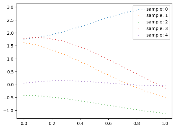
Let’s recall on the steps we need to compute several samples from a GP characterized by an RBF kernel using a python script example:

    import numpy as np
    from sklearn.metrics.pairwise import pairwise_kernels as kernel
    import matplotlib.pyplot as plt

    seeds = [0,1,2,3,4]
    for seed in seeds:
        np.random.seed(seed)
        # Define sample size
        N = 50
        # Define domain to sample
        X = np.linspace(0,1,N)
        # Compute kernel matrix using e.g. RBF kernel
        C = kernel(X.reshape(-1,1), metric='rbf') + 1e-6*np.eye(N)
        # Get Cholesky factor of C
        L = np.linalg.cholesky(C)
        # Get a normal vector
        Z = np.random.normal(size = (N,))
        # Compute sample from f ~ GP(0,RBF)
        f = L @ Z
        # Plot samples
        plt.scatter(X,f, s = 0.5, label = f'sample{seed}')
        plt.legend(loc = 'upper right')
    plt.show()

Eigendecomposition of a GP

If \(C = Q \Lambda Q^\top\) then \(C^{1/2} = Q \Lambda^{1/2} Q^\top\). Let’s investigate then on the distribution of \(C^{1/2}Z\), which by the calculation before is given by

Here notice that by properties of Gaussian random vectors,

Thus, \(f \overset{d}{=} C^{1/2} Z \overset{d}{=} Q \Lambda^{1/2} W\) where \(W \sim N(0,I_N)\). And if \(W = (w_1,\dots,w_N)^\top\) is \(N-\)dimensional then explicitly we have

where we recall that each \(w_j \sim N(0,1)\).

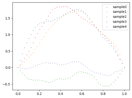
For instance, if we take \(\lambda_j = \frac{1}{j^{2\alpha}}\), \(q_j = \begin{pmatrix}\sin(j \pi x_1) \dots \sin(j \pi x_N)\end{pmatrix}^\top\) and \(w_j \sim N(0,1)\) one can sample a pinned GP with regularity \(\alpha\) using a python script example:

    alpha = 2
    seeds = [0,1,2,3,4]
    for seed in seeds:
        np.random.seed(seed)
        # Define sample size
        N = 50
        # Define domain to sample
        X = np.linspace(0,1,N)
        # sine matrix
        Q = np.array([np.sin(j*np.pi*X) for j in range(1,N+1)]).T
        # e-vals
        L_SQRT = np.diag([j**(-alpha) for j in range(1,N+1)])
        # W
        W = np.random.normal(size = (N,)) 
        # Compute sample
        f = Q @ L_SQRT @ W
        # Plot sample
        plt.scatter(X,f, s = 0.5, label = f'sample{seed}')
        plt.legend(loc = 'upper right')

References:

• For the connections between Gaussian Process Regression, kernel ridge regression and RKHS methods we followed this:

[1] Kanagawa, Motonobu, et al. “Gaussian processes and kernel methods: A review on connections and equivalences.” arXiv preprint arXiv:1807.02582 (2018).

• For a classical treatment of the use of GPs in machine learning we are inspired by:

[2] Williams, Christopher KI, and Carl Edward Rasmussen. Gaussian processes for machine learning. Vol. 2. No. 3. Cambridge, MA: MIT press, 2006.